Understanding Snakemake

Each day, data scientists, computational biologists, astronomers, and other folks that spend far too much time in front of a computer screen spend hours doing somewhat horrible, monotonous tasks. Scientific programming, when done right, is supposed to prevent us from doing these monotonous tasks, and this is certainly true when we compare what we do today to what the tireless programmers and human computers of the 1950s did: inverting matrices by hand, writing code to calculate the t-statistic and corresponding p-value, and so forth. All of these monotonous tasks, thankfully, are implemented now in modern libraries like BLAS/LAPACK, GNU Scientific Library, numpy, R, eigen, etc. However, the problem has just shifted: today’s monotonous tasks are tidying messy data, applying a linear model to tens of thousands of data sets, or assessing prediction accuracy across statistical model parameters using cross validation.
Some of these monotonous tasks have been made easier by very clever abstractions. Consider R’s tidyverse, which has simplified numerous monotonous tasks most R users do by realizing these tasks fit a pattern: import data, tidy that data, explore the data, and communicate the findings (see Hadley Wickham’s book R for Data Science). Similarly, scikit-learn has slick classes to do the tedious task of model selection. Additionally, data projects usually involve lots of repetitive file system work: downloading datasets, running command line tools to pre-process raw data, running simulation software, etc. These tasks are often repetitive because, throughout the course of a project, you’ll likely need to re-run the same steps multiple times. On page 9 of my book Bioinformatics Data Skills I explain why:
You will almost certainly have to re-run an analysis more than once, possibly with new or changed data. This happens frequently because you’ll find a bug, a collaborator will add or update a file, or you’ll want to try something new upstream of a step. In all cases, downstream analyses depend on these earlier results, meaning all steps of an analysis need to be re-run.
What abstraction and accompanying software tools allows us to avoid these humdrum repetitive tasks we do in the Unix shell? Make and Snakemake.
Make
I think the best way to learn Snakemake (our ultimate goal) is to first get a rough sense of how its predecessor, Make, works. I still use Make for simple tasks, and you’ve already likely used it to compile software at some point. Make is a software tool and language that’s been around since 1976, and is still widely used. Originally it was designed as a way to automate building software, but the central problem of compiling software is quite like the problem described above: some input file will change, and all downstream files that depends on this file needs to be updated by re-running code. Compiling software is relatively time consuming, so Make’s designers took advantage of a simple idea: if we declare what files depend on other files, we only need to run the steps downstream of the files that have changed. In computer science lingo, we write out the code compiling steps as a directed acyclic graph, and only the paths connected to a changed file need to be re-run. This will become clear with some examples.
First, Make (the software) looks for file named Makefile in a directory when we run the make command1. In a Makefile, we specify the rules describing the steps to run to turn input files into output files. Specifically, a Makefile consists of:
A target, the thing to build with this rule. This is the output file.
A single or list of dependencies files. These are the files needed by the rule to create the target.
Commands, or the list of Unix commands needed to convert the dependencies into the target.
The format of a rule is:
file_target.txt: dependency_1.txt dependency_2.txt
    unix_command dependency_1.txt dependency_2.txt > file_target.txt
Note that the command line must begin with a tab character, not spaces. Make’s a bit of a grumpy about this. Still, Make is quite clever, in that it will only re-run each rule if (1) the input files changed, or (2) the target does not exist and needs to be generated.
I still use Make for the simplest redundant file tasks: usually downloading data from the web, and doing some minimal pre-processing. For example, in a recent project I wanted to download the genome of Drosophila melanogaster and create a file containing the lengths of all the sequences using bioawk. Here’s what a Makefile running these steps looks like2:
all: Dmel_BDGP6.28_seqlens.tsv

Drosophila_melanogaster.BDGP6.28.dna.toplevel.fa.gz:
  wget ftp://ftp.ensembl.org/pub/release-99/fasta/drosophila_melanogaster/dna/Drosophila_melanogaster.BDGP6.28.dna.toplevel.fa.gz

Dmel_BDGP6.28_seqlens.tsv: Drosophila_melanogaster.BDGP6.28.dna.toplevel.fa.gz
  # note we need the double dollar signs here, since the $ indicates a variable in Make
  bioawk -c fastx '{print $$name "\t" length($$seq)}' Drosophila_melanogaster.BDGP6.28.dna.toplevel.fa.gz > Dmel_BDGP6.28_seqlens.tsv
You can give this a try for yourself by copying and pasting this into a file called Makefile in an empty directory (or downloading it from Github) and typing:
$ make allThis looks for a file named Makefile, and runs the all target. Note that Make is a declarative language, meaning it doesn’t execute code from top to bottom like a normal program’s control flow. Instead you declare what needs to be done, and it executes things in the right order. Stepping through the Makefile code, there are three rules, which I’ll explain in the order Make works through them:
all, which is the primary target. It’s the starting place; typingmake alltells Make to createall’s dependencies. In this case, there’s only one dependency:Dmel_BDGP6.28_seqlens.tsv.Now, make is looking for
all’s dependency,Dmel_BDGP6.28_seqlens.tsv. Since this file does not exist, Make looks for a rule to create this target. It finds this rule, but this rule requires the fileDrosophila_melanogaster.BDGP6.28.dna.toplevel.fa.gz. This file isn’t in this directory yet either, so Make goes looking for a rule to build that.The second rule (after
all) declares how to generateDrosophila_melanogaster.BDGP6.28.dna.toplevel.fa.gz. This target requires no dependencies, so Make proceeds straight into executing the rule: usewgetto download a file from the web.One this file downloads, the dependency for the
Dmel_BDGP6.28_seqlens.tsvfile is available. Make, working backwards, runs this rule now, calling bioawk to summarize the sequence lengths of this genome. This generates the fileDmel_BDGP6.28_seqlens.tsv.Finally, make has satisfied dependency of
all:Dmel_BDGP6.28_seqlens.tsv. Since it’s got everything it needs, it quits.
The real magic is what happens if we delete Dmel_BDGP6.28_seqlens.tsv, or change Drosophila_melanogaster.BDGP6.28.dna.toplevel.fa.gz. Unlike a bash script, which will re-run everything start to finish, Make will only re-run what it needs to build files depending on the changed files:
$ rm Dmel_BDGP6.28_seqlens.tsv
$ make all  # since the genome hasn't been changed or deleted, only the last rule is run!
bioawk -c fastx '{print $name "\t" length($seq)}' Drosophila_melanogaster.BDGP6.28.dna.toplevel.fa.gz > Dmel_BDGP6.28_seqlens.tsv
We can emulate changing an input file in this example by using touch to change the timestamp of the Drosophila_melanogaster.BDGP6.28.dna.toplevel.fa.gz file:
$ touch  Drosophila_melanogaster.BDGP6.28.dna.toplevel.fa.gz
$ make all  # runs all downstream steps
bioawk -c fastx '{print $name "\t" length($seq)}' Drosophila_melanogaster.BDGP6.28.dna.toplevel.fa.gz > Dmel_BDGP6.28_seqlens.tsv
Make gets a lot, lot more complicated than this simple example. The language is rich, but its a rather tedious language for all about the simplest tasks. As you use Make more, I’d recommend learning more about its automatic variables, which allow us to avoid redundantly typing out target and dependency filenames. The two I use most are $@, which is a placeholder for the filename of the target, and $<, the name of the first prerequisite. This would simplify our earlier Makefile like so3:
all: Dmel_BDGP6.28_seqlens.tsv

Drosophila_melanogaster.BDGP6.28.dna.toplevel.fa.gz:
  wget ftp://ftp.ensembl.org/pub/release-99/fasta/drosophila_melanogaster/dna/Drosophila_melanogaster.BDGP6.28.dna.toplevel.fa.gz

Dmel_BDGP6.28_seqlens.tsv: Drosophila_melanogaster.BDGP6.28.dna.toplevel.fa.gz
  bioawk -c fastx '{print $$name "\t" length($$seq)}' $< > $@
Finally, it’s worth mentioning that Make is trivially parallelizable. Since Makefiles describe the chain of rules needed to create a file, indepenent chains can be run across different cores simulultaneously. The example above is too simple to run steps in parallel, but if did have independent chains that could be run independently, we’d do this with:
$ make -j 4 # run the Makefile on 4 coresMake is definitely finicky and old; after all, it first emerged in 1974. I still use Make for the simplest of data downloading and pre-processing tasks, much like Mike Bostock describes. While there was a time when I would dig deep into the Make documentation, using Make’s functions to write complicated Makefiles to process hoards of data, now I prefer Snakemake.
Snakemake
Snakemake is a new, Python-based build automation software program. Unlike Make, which was intended to be used to automate compiling software, Snakemake’s explicit intention is to automate command line data processing tasks, such as those common in bioinformatics. You can install Snakemake with Conda (instructions here). Much like Make, running the command line program snakemake looks for a Snakefile, named Snakefile in the directory. And much like Make, the format of the Snakefile has rules defined by targets (known in Snakemake as outputs), dependencies (Snakemake calls these inputs), and rules (and a lot more is possible here with Snakemake, as we’ll see). Let’s translate our earlier Makefile to a Snakefile4:
rule all:
  input:
    "Dmel_BDGP6.28_seqlens.tsv"

rule genome:
  output:
    "Drosophila_melanogaster.BDGP6.28.dna.toplevel.fa.gz"
  shell:
      "wget ftp://ftp.ensembl.org/pub/release-99/fasta/drosophila_melanogaster/dna/Drosophila_melanogaster.BDGP6.28.dna.toplevel.fa.gz"

rule seqlens:
  input:
    "Drosophila_melanogaster.BDGP6.28.dna.toplevel.fa.gz"
  output:
    "Dmel_BDGP6.28_seqlens.tsv"
  shell:
      """bioawk -c fastx '{{print $name "\t" length($seq)}}' {input} > {output}"""
The key changes are:
Slightly different rule format, and all rules are named (e.g.
all,genome, etc.).Filenames and shell commands must be quoted (note that Python’s triple quotes can be used to avoid escaping quotes in cases where single and double quotes are used in the rule).
Rules running shell commands are specified in
shellblocks. Snakemake also supports running Python inrunblocks.Rather than awkward special variables like Make’s
$@and$<, Snakemake uses Python’s formatted strings (i.e. the braces in the last line) and clear names like{input}and{output}. However, since braces are now special in Snakemake, we need to escape them when using them in our bioawk line; a literal brace is specified by using two of them, e.g.{{and}}(this is analogous to how we had to escape the$in Make by using$$!).
This is then executed much like a Makefile. Before executing it though, let’s do a dry run with snakemake --dryrun or snakemake -n. This doesn’t execute any steps, it just shows what Snakemake would do if run5:
$ snakemake --dryrun
Building DAG of jobs...
Job counts:
    count   jobs
    1   all
    1   genome
    1   seqlens
    3

[Thu Mar  5 11:37:28 2020]
rule genome:
    output: Drosophila_melanogaster.BDGP6.28.dna.toplevel.fa.gz
    jobid: 2


[Thu Mar  5 11:37:28 2020]
rule seqlens:
    input: Drosophila_melanogaster.BDGP6.28.dna.toplevel.fa.gz
    output: Dmel_BDGP6.28_seqlens.tsv
    jobid: 1


[Thu Mar  5 11:37:28 2020]
localrule all:
    input: Dmel_BDGP6.28_seqlens.tsv
    jobid: 0

Job counts:
    count   jobs
    1   all
    1   genome
    1   seqlens
    3
This was a dry-run (flag -n). The order of jobs does not reflect the order of execution.
Now, let’s execute these steps – on the command line, enter:
$ snakemakeUnlike Make, Snakemake has a really nice progress reporting (I’ve omitted this output above for brevity).
Using Expand to Build up all Filesnames and Parameter Combinations
The real strength of Snakemake is how easy it makes applying rules across multiple files that share a similar filename structure (this is why it is so important to have a consistent file name scheme!). I’ll demonstrate this incrementally with a few Snakefiles, which because we can program in Python with Snakemake, allow us to see what’s happening with print() statements. First consider this Snakefile6:
chrom_filename = "Drosophila_melanogaster.BDGP6.28.dna.chromosome.{chrom}.fa.gz"

chroms = ['2L', '2R', '3L', '3R', 'X', '4']

chrom_fa_files = expand(chrom_filename, chrom=chroms)

print(chrom_fa_files)
Now, rather than downloading the entire Drosophila melanogaster genome, we’re going to download some individual chromosome sequences7. We exploit these well-named files, and build all the chromosome sequence filenames that need to be downloaded programmatically with Snakemake’s powerful expand() function. expand() builds a list of strings by replacing the string {chrom} in chrom_filename with each of the chromosome names in the chroms list. We use print() on the last line to look at the resulting list of filenames.
While above we used expand() to build up chrom_fa_files, populating it with values from just the chroms list, it works with more than one input list too, and generates all combinations (a Cartesian Product) of the input values. This makes expand() exceedingly powerful because it can be used to build up all possible parameter combinations for a series of simulations. Consider8:
import numpy as np
Ns = [100]
selcoefs = 10**np.linspace(-3, -1, 3)
rbps = 10**np.linspace(-8, -7, 2)
nreps = np.arange(20)

sim_results_pattern = "sim_{N}N_{selcoef}s_{rbp}rbp_{rep}rep.tsv"

sim_results = expand(sim_results_pattern,
                     N=Ns, selcoef=selcoefs,
                                          rbp=rbps, rep=nreps)

print(sim_results)
Running this, we see we have a list of all results files for all parameter combinations:
$ snakemake
['sim_100N_0.001s_1e-08rbp_0rep.tsv', 'sim_100N_0.001s_1e-08rbp_1rep.tsv',
 'sim_100N_0.001s_1e-08rbp_2rep.tsv', 'sim_100N_0.001s_1e-08rbp_3rep.tsv',
 'sim_100N_0.001s_1e-08rbp_4rep.tsv', 'sim_100N_0.001s_1e-08rbp_5rep.tsv',
  ...
 'sim_100N_0.1s_1e-07rbp_14rep.tsv', 'sim_100N_0.1s_1e-07rbp_15rep.tsv',
 'sim_100N_0.1s_1e-07rbp_16rep.tsv', 'sim_100N_0.1s_1e-07rbp_17rep.tsv',
 'sim_100N_0.1s_1e-07rbp_18rep.tsv', 'sim_100N_0.1s_1e-07rbp_19rep.tsv']
Building DAG of jobs...
Nothing to be done.
Complete log: /Users/vinceb/projects/snakemake-tutorial/example-05/.snakemake/log/2020-03-05T190027.307441.snakemake.log
There’s nothing special about by my file name scheme here, though it is one that I often use. The filenames could be parsed by downstream programs so the parameters are known, but I prefer usually to have the simulation software write a metadata string at the top of the results files (e.g. as a comment line a TSV/CSV beginning with #).
Using Wildcards
In the previous section, we automatically created a bunch of filenames of simulation results we want after running all our simulations, representing all combinations of parameters. Now, we need to write a rule that describes how to actually run all these simulations and pass the appropriate parameters to the command line tool responsible for running the simulations. What’s elegant about Snakemake is that since each file is the result of running a simulation once with particular parameters, we can write one special general rule that describes how to generate all the simulation results. The trick to do this is to use wildcards.
Understanding wildcards was, for me, the hardest part of understanding Snakemake. They’re just magic enough to be confusing, but also really useful. The best way to grok wildcards is to understand that they match parts of a rule’s output file. I think it’s easier to explain this through a simple example, after which we’ll continue the simulation example described above.
Here’s a simple example of wildcards9:
results = "file_{sample}.txt"

all_results = expand(results, sample = [1, 2, 3])

rule all:
  input:
    all_results

rule sims:
  input:
  output:
    "file_{sample_name}.txt"
  run:
    with open(output[0], 'w') as f:
      f.write(f"the sample name is {wildcards.sample_name}")
Note that rather than using the shell block, we’re using a run block which is just pure Python code – this is a beautiful feature of Snakemake. In this block, the variable output is automatically set by Python, and is a list of all files in output. However, since we’re using wildcards, Snakemake is passing in the files from all_results one at a time, so this list contains just a single file. We grab the only file in the list, output[0] and open it for writing. In that file, we write the contents of {wildcards.sample_name}, which Snakemake also automatically sets for each output filename.
If this is still unclear, it’s important to remember that Snakemake is working backwards. The all target is first run, and Snakemake looks for this rule’s inputs: the list of files in all_results. Then, since these files don’t exist, Snakemake looks for a rule to generate them. The sims rule’s output matches the filenames needed – "file_{sample_name}.txt" is treated like "file_*.txt" would be by Unix. The difference is that the matching section is assigned to wildcards.sample_name and can be used by the rule’s shell or run block.
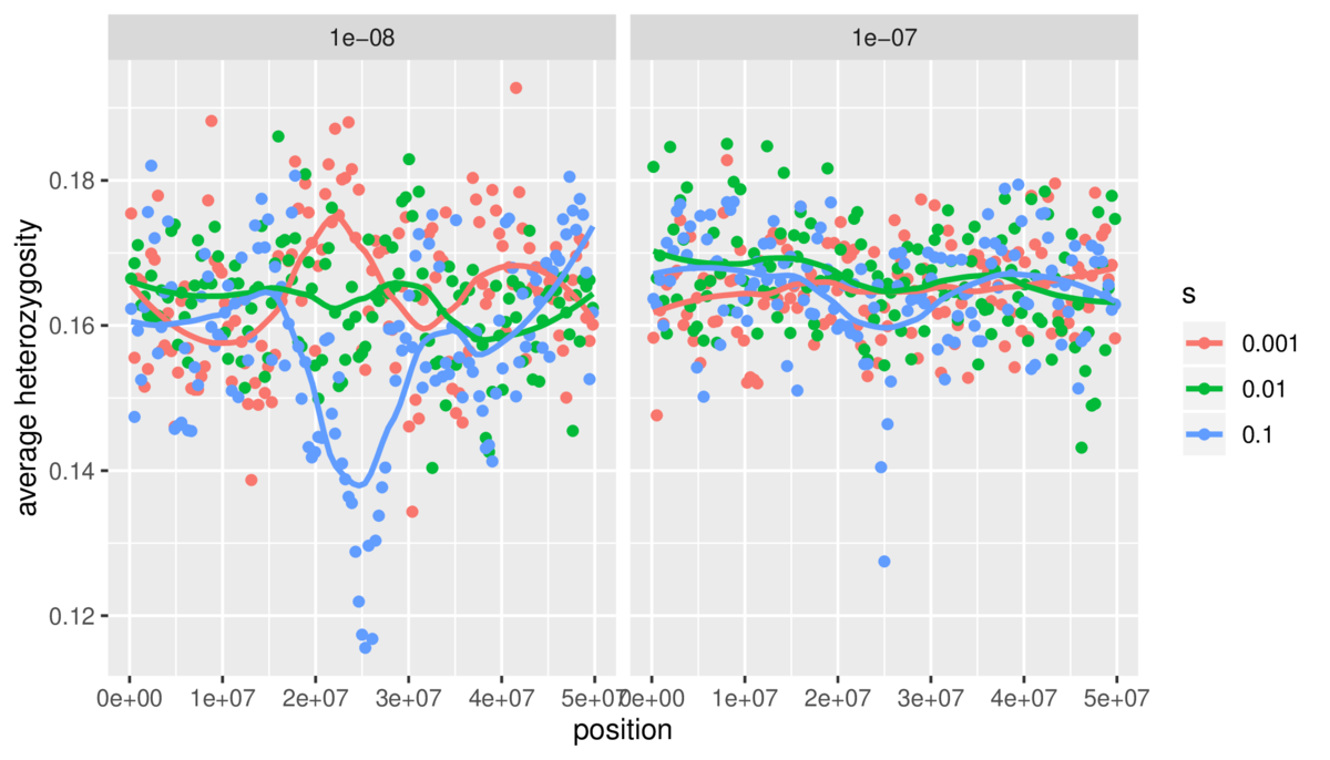
With this simple example hopefully making wildcards clearer, let’s continue our simulation example. For this example, I use the population genetics forward simulation software SLiM from the Messer Lab, but the basic idea extends broadly to bioinformatics and data science tasks. I’m simulating evolution of a stretch of chromosome, where selected mutations pop in the population, but only in a small region (emulating a gene) in the middle of the chromosome. The details of the simulation are on Github, and I use the Snakemake file to try different parameters, in this case selection coefficients and the level of recombination. I also use Snakemake to generate a lot of independent replicate results. The Snakemake file10 looks like:
import numpy as np
Ns = [100]
selcoefs = 10**np.linspace(-3, -1, 3)
rbps = 10**np.linspace(-8, -7, 2)
nreps = np.arange(40)

sim_results_pattern = "sim_{N}N_{selcoef}s_{rbp}rbp_{rep}rep.tsv"

sim_results = expand(sim_results_pattern,
                     N=Ns, selcoef=selcoefs,
                     rbp=rbps, rep=nreps)

rule all:
  input:
    sim_results

rule sims:
  input:
  output:
    sim_results_pattern
  shell:
    # split across two lines, to make this easier to fit on screen:
    ("slim -d s={wildcards.selcoef} -d rbp={wildcards.rbp} " +
     "-d N={wildcards.N} -d rep={wildcards.rep} sim.slim")
Here, Snakemake captures the wildcards and passes them directly into the command line call to SLiM. We can run this across four cores with:
$ snakemake --cores 4This creates a lot of simulation results. Processing these files isn’t within the scope of this tutorial, but you can see the R script I used to do so on Github. Additionally, I’ve included another Snakemake file for this example showing how Snakemake can also be used to run scripts to make figures, using the simulation results generated by another part of Snakemake. It’s Snakes all the way down! Our final result is a figure:
Future
I hope this has convinced you that Snakemake is a powerful tool that should be in your computational toolbox, and it is clearer how some of the more powerful features of Snakemake (expand() and wildcards) work. For what it’s worth I still use Make for small tasks, and will continue to do so.
While I use Snakemake a fair amount now, I expect this to continue to increase. Why? Once you become acquainted with Snakemake, you start to see increasingly many areas in a project you can use it in (e.g. generating figures, parsing collating raw data, running unit tests). Snakemake becomes fun to use because it prevents the monotony of running the same steps repeatedly in a project. I think too many years coding up analyses have made me realize that 70% of the computational work of an analysis or project is the same as every other project. This shared component of computational work is not intellectually stimulating, and if some tool or library can serve as a higher-level abstraction that makes these repetitive tasks easier, it frees up time to work on intellectually stimulating parts of a project – the stuff I enjoy more. Hopefully Snakemake will help you do more monotonous data tasks in less time with less effort too.