Introducing camdl: engineering rigor for stochastic compartmental modeling
Disclosure: camdl is an open-source project I am developing at the Institute for Disease Modeling (Gates Foundation). I'm cross-posting here from internal channels since the project is public; the views expressed are my own and don't represent IDM or the Foundation.
Engineering scientific software is a different problem than general software engineering. The most consequential bugs in scientific code don’t crash loudly — they produce valid-looking results that get published in peer-reviewed papers. In 2006, Geoffrey Chang retracted five papers from Science, J. Mol. Biol., and PNAS because a sign-flip in his homemade data-reduction script had silently inverted the hand of his protein structures. Or take a favorite scientific bug example in genomics: more than a decade after Excel’s gene-symbol-to-date autoconversion was first documented , roughly a fifth of published supplementary tables still have it. And these are just the cases that got caught — the silent failures are by definition the ones that don’t.
The stakes of this default may be low when scientific code is just producing a figure for a paper. But in computational epidemiology, our software isn’t just producing an artifact, it’s informing decision-making in public health: outbreak responses, vaccination strategies, or major investments. The most consequential bugs in this domain aren’t crashes, they’re silently erroneous code that creates pernicious problems: trajectories that look plausible but lead decision makers astray — a per-capita rate written where the propensity needed a population-level one, a unit slip that survives review, uncertainty that should be conveyed but is silently dropped, a calibration that looks converged but isn’t. IDM’s pioneering agent-based simulator EMOD has a codebase that’s roughly 24% tests — a great early example of an engineering investment in scientific software long before it was standard. Eliminating entire classes of bugs should be, in my view, a central engineering goal of writing good epidemiological software.
A central challenge in the design of scientific software is the labor specialization of its users. An epidemiologist may spend a decade studying immunology, disease dynamics, vaccinology, etc., building domain expertise that is invaluable when it comes to producing good models. But such specialization has an unavoidable opportunity cost: every year spent on transmission dynamics is a year not spent on learning software engineering best practices, statistical inference algorithms, numerical analysis, compiler design, or software architecture. This problem is especially acute in low- and middle-income public-health offices, where research groups are often small and a single epidemiologist plays both modeler and software engineer — not for lack of capability, but for lack of the resources that wealthier research environments take for granted.
Since joining IDM, I’ve been curious whether domain-specific languages (DSLs)
could lower this engineering burden — letting modelers do rigorous inference
without first having to become rigorous software engineers. A DSL is a small
programming language purpose-built for one problem domain. The model’s code is
then just a declaration of the scientific model, written in a syntax that
reads like the whiteboard math you’d share with a colleague (e.g. infection : S --> I @ beta * S * I / N), and the runtime is the separate program that
actually executes it. A compiler1 sits between the DSL and the
runtime: it reads the model declaration, compiles it, checking extensively for
errors, and emits an intermediate representation (IR) the runtime consumes to
actually execute the simulation. With this DSL-compiler-IR architecture, the
modeler never needs to write the finicky, bug-prone code underneath — the
state-update loop, the propensity evaluator, the particle filter, the gradient
code. Instead, they describe the model; the compiler and runtime handle the
rest. Most scientific software tangles model and runtime implementation in one
script; the DSL-compiler-IR architecture keeps them apart. The closest
analogues are Stan
in statistics and
odin
for compartmental ODE modeling in R.
Both are excellent at what they do, and both heavily influenced camdl’s design:
Stan showed how far a probabilistic DSL with a serious compiler can go; odin
showed that a small, focused DSL can transform how a community writes its
models. camdl is in their lineage.2
But the DSL is only part of the answer. With camdl, I wanted the compiler doing more work to validate models — a goal that’s only gotten more urgent as coding agents start writing more model code (especially when the work is upstream of decision making). The compiler-level checks camdl does catch many mistakes regardless of who introduced them, human or agent; in both cases, the user gets friendly error, warning, or info messages. The compiler checks dimensions and units like a type system, differentiates rate expressions symbolically so inference gets exact gradients without an autodiff dependency, expands stratified models from a single declaration, and rules out subtle discretization bugs before anything runs.
I also wanted the runtime on the other side to match that effort: a full simulation and inference framework, with four simulation backends sharing one compiled model (Gillespie, tau-leaping, Euler-multinomial / chain-binomial, ODE) and backend compatibility checked before any step is taken, particle-filter methods that are standard for these inference problems (IF2 for MLE; PGAS+NUTS — a Gibbs split that updates latent trajectories with PGAS and parameters with NUTS — and PMMH for Bayesian posteriors), convergence gates that catch and flag bad model fits rather than passing them silently through, and content-addressable provenance so re-running a fit is a cache hit instead of a fresh run.
The compiler is written in OCaml (the same language Stan’s compiler uses, a fact I discovered only after I’d already made the same choice!), whose algebraic data types and pattern matching are what make serious compiler work tractable; the simulation runtime is in Rust, for memory safety and the performance this kind of engine needs.
Overall, camdl is my attempt to engineer a robust stochastic compartmental modeling framework around DSL architecture and cutting-edge statistical algorithms for model fitting. camdl isn’t a proof-of-concept: it has been technically validated by reproducing the findings of published disease models — He et al.’s 2010 fit of London’s measles data and the classic UK boarding school influenza outbreak — and ships with 1,204 tests, including continuous validation against pomp, scipy, and Kermack–McKendrick closed-form solutions, all run as CI gates that block merges on regression. The Garki Project Malaria Model and the Dhaka cholera dataset from King et al. (2008) are currently in flight as further external validations.
The rest of this post is a tour. I’ll start with what a real, fit-validated model looks like in camdl (the He et al. (2010) London measles SEIR, the canonical particle-filter benchmark) then walk through stratification at compile time, the compiler-level catches that rule out the silent bugs I described above, surveying the likelihood surface before committing to a fit, the scout / refine / validate calibration pipeline with its mandatory convergence gates, and the inference algorithms camdl ships.
A real model, written like the math
Here is a fragment of He, Ionides & King (2010) — the canonical particle-filter measles benchmark, fit to London weekly notifications 1950–1964, externally validated against pomp — written directly in camdl:
# He et al. (2010) London measles SEIR
# Full model: 138 lines — see he2010 vignette

forcing {
  pop       : interpolated 'count { data = "covariates.tsv", value_col = population }
  birthrate : interpolated 'count { data = "covariates.tsv", value_col = birthrate }
  school    : periodic 'ratio { period = 365.25 'days, step = 1 'days, on = [7:100, 115:199, 252:300, 308:356] }
}

let seas = 1.0 - amplitude + amplitude * (1.0 + 0.2411 / 0.7589) * school(t)

transitions {
  infection : S --> E  @ overdispersed(beta_base * seas * S * ((I + iota)^alpha) / pop(t), sigma_se)
  latency   : E --> I  @ sigma * E
  recovery  : I --> R  @ gamma * I
  birth     : --> S    @ deterministic((1.0 - cohort) * birthrate(t) * pop(t) / 365.25)
  # ... + per-compartment mu deaths
}

events {
  cohort_entry : add(S, cohort * birthrate(t) * pop(t))  every 365.25 'days at_day 258
}

observations {
  weekly_cases : {
    projected  = incidence(recovery)
    every      = 7 'days
    likelihood = normal(mean = rho * projected,
                        sd   = sqrt(rho * projected * (1 - rho + psi^2 * rho * projected)))
  }
}
This model has it all: time-varying covariates, UK school-term forcing, overdispersed environmental noise on the force of infection, a once-per-year cohort pulse, and the He et al. heteroscedastic observation likelihood. All of these model features are encoded using features of the camdl language; all are declarative, all compiler-checked. The full 138 lines of camdl (only 78 lines of actual code; the rest is for human-readability) build a model that pomp’s reference implementation expresses in 238 lines of mixed R, C Csnippet, and shell-wrapper glue, most of which is plumbing rather than science:
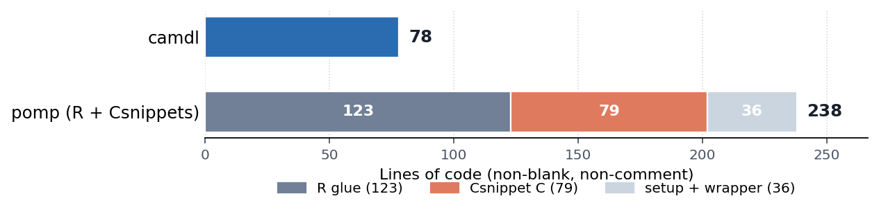
# for camdl/R/shell, // for C inside Csnippets). pomp’s bulk is split into the R model code, the C Csnippets it embeds, and the setup + wrapper scripts that drive it.Another feature of this architecture is the sharp responsibility split: the
modeler is responsible for specifying the model in a .camdl file, and camdl
and its developers are responsible for everything after: the compilation to IR,
the runtime faithfully implementing the model’s simulation, and the inference
stack working properly. If a compiling model produces a trajectory inconsistent
with its declared semantics, that’s a camdl bug — not a modeler bug. By the
DSL-compiler-IR architecture, the modeler cannot ever be responsible for an
implementation bug, because they’re never writing the implementation code.
Stratification is a compiler pass
The He et al. (2010) model above is one-dimensional; it models a single SEIR for all of London. But often the models researchers actually want to fit for policy work are not this simple: they’re stratified by age, by space, by risk group, by vaccination status.
Previously, adding these extra dimensions of realism could be a burden on the modeler — especially since dimensions compound multiplicatively. For example, \(P\) patches and \(A\) age groups create \(P \times A\) compartments, each of which needs careful, tedious and error-prone bookkeeping when writing out the transition logic; add a third stratifier and that count multiplies again. Suppose a modeler spends a day carefully coding one of these up, and a colleague then suggests fitting an alternate model with an extra risk-group dimension. Such a model comparison activity is exactly the type of workflow that leads to better modeling, and thus better decisions; camdl’s philosophy is that we want to encourage better modeling by reducing frictions that make creating and fitting alternative models painful, slow, and fragile. Adding an extra dimension could easily increase model code by a large factor; moreover, every new line is a place for a typo to silently lead to science bugs like encoding the wrong transmission propensity for a given patch, age, risk group compartment. In pomp, exploring an alternative model structure would be hundreds of lines of C snippets; in NumPyro it’s vectorized indexing you write and own correctness for.
By contrast, camdl’s DSL is designed to make stratification something the
compiler does for you. You declare a dimensions {} block and a stratify
directive, and the compiler expands the base model into the full Cartesian
product before anything else runs:
dimensions { age = [child, adult] }
stratify(by = age)

let N_local[a in age] = S[a] + E[a] + I[a] + R[a]

tables {
  C_age : age × age = [[12.0, 4.0], [4.0, 8.0]]   # contact matrix
}

transitions {
  infection[a in age] : S[a] --> E[a]
    @ beta * S[a] * sum(b in age, C_age[a, b] * I[b] / N_local[b])
  progression[a in age] : E[a] --> I[a]  @ sigma * E[a]
  recovery[a in age]    : I[a] --> R[a]  @ gamma * I[a]
}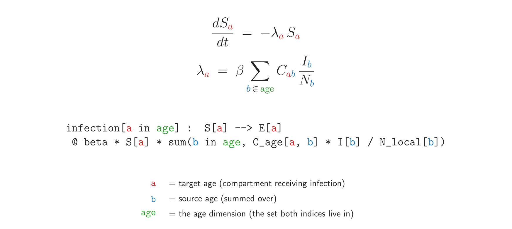
age (green). Every red age index a in
the math has a red a index with the same role in the camdl, and ∑_{b ∈ age}
matches sum(b in age, ...) exactly.That’s an entire age-stratified SEIR in camdl. The compiler expands it to 8
compartments and 6 transitions, dim-checks the contact-matrix indexing (a
typoed dimension key is a compile error, not a silent zero), and hands the
runtime an IR that looks no different from the unstratified case. Surveying,
fitting, and held-out validation all work on the expanded model unchanged. The
same pattern composes: add a second stratify(by = space) and the compiler
builds the full age × space product, with the same guarantees.
A compiler doing what scripts can’t
When I was first implementing the He et al. (2010) London measles model in camdl,
there was a 12-nat difference in the log-likelihood against pomp that had me
scratching my head for two days. The ultimate cause was a single line: (1 - exp(-rate * 1 'days)) — a propensity that a coding agent wrote that’s
correct only when the runtime integrator step dt happens to equal 1 'day.
But if a user were to run the model with any other dt, the rate would be
incorrect. Surprisingly, this bug passed synthetic data parameter recovery,
since the same bias appeared on both sides of the simulate/fit loop. In
developing camdl, my design philosophy is to study these types of
tricky-to-catch bugs and engineer them away.
In this case, a user isn’t wrong per se to write a model this way (it passes
dimensional analysis), it’s just a very fragile way to encode the dynamics. But
this is also a target for compiler-based checks. Here, the fix was a compiler
lint (L401) that catches the AST shape, points at the literal, and suggests
the modeler use the dt primitive that makes the same expression
dt-invariant. The bug could not have been surfaced without compiler-level
inspection of the expression tree. In my view, it’s a strong argument for
building modeling language compilers: we can leverage compilers to catch
fragile choices in modeling user-space.
That’s the kind of bug camdl’s compiler is built to rule out. As stated earlier, the most consequential modeling bugs are not crashes; they’re unit slips, dimension errors, and typos that produce trajectories that look plausible but are quietly wrong. The camdl compiler catches each class before anything runs. User testing will undoubtedly surface more ways in which users unintentionally build fragile models — each of which becomes a fun engineering challenge: how can we make a model compiler catch this?
Below are some more examples of what bug classes the camdl compiler can catch.
Units. Tick-prefixed annotations ('days, 'weeks, 'per_year) are
first-class in camdl (unit mismatches are a notorious source of expensive
errors
);
the compiler converts to the model’s specified time_unit. When the user
specifies a unit in a way that is subtle or ambiguous, the camdl compiler
refuses rather than guessing:
$ camdl check bad_unit.camdl

error[E107]: ambiguous unit literal after '/': the unit suffix binds
to the adjacent number, not the whole expression. Use parentheses:
(20 / 100_000) 'per_year, or pre-compute: 0.0002 'per_year

  ┌─ bad_unit.camdl:9:17
  │
9 │  let mu : rate = 20 / 100_000 'per_year
  │                  ~~~~~~~~~~~~~~~~~~~~~^
Dimensions. Every expression in camdl carries an (P, T) population-time
dimensional tuple. For example, compartmental counts are (1, 0), per-capita
rates are (0, -1), population-level rates are (1, -1). When camdl compiles
a model, its dim-checker propagates these through every operation and rejects
mismatched dimensions. This catches a very common class of modeling user-space
bugs — writing a per-capita rate where a total propensity is needed:
$ camdl check bad_dimension.camdl

error[E300]: transition 'infection' rate has wrong dimension

  rate = ((beta * I) / (S + I + R))
  expected dimension: P*T^-1 (population-level rate)
  got dimension: T^-1 (per-capita rate)
In pomp, NumPyro, or hand-rolled R, the second form compiles silently and produces trajectories where infection silently happens at entirely the wrong rate.
Names. The camdl compiler also catches typos that would silently introduce a new variable:
$ camdl check bad_name.camdl

error[E100]: undeclared name 'Q'

   ┌─ bad_name.camdl:11:33
   │
11 │   recovery  : I --> R @ gamma * Q
   │                                 ^
  = hint: check spelling, or add a declaration in
    compartments/parameters/let/tables
Overall, camdl’s contribution is engineering rigor, enabled by having a specialized compiler. Typos, unit mismatches, and per-capita-vs-propensity confusion are exactly the class of bug a compiler can rule out, so scientific scrutiny can focus on the science.
A frame I keep coming back to here, borrowed from a personal interest in the Toyota Production System after reading Ohno’s Toyota Production System: Beyond Large-Scale Production : this is poka-yoke , which translates roughly to error-proofing at the source. This ingenious idea can be applied to scientific model building via well-engineered software.
Surveying the likelihood surface before you fit
The hardest fitting bugs aren’t the ones where the chain fails to converge — those at least tell you something is wrong. They’re the ones where a single optimization run confidently points a researcher to one plausible parameter point among an unseen sea of equally plausible alternative parameters. While multi-start optimizations, parallel MCMC chains, and convergence diagnostics can surface these identifiability issues (and all are built into camdl), I wanted an exploratory data analysis (EDA) approach to catching these types of model fitting pathologies earlier: two parameters trading off along a ridge, a parameter pinned at a bound you set too tight, a region of parameter space the data simply cannot distinguish from another.
So before any camdl fit run, I almost always reach for camdl survey — a
diagnostic that maps the likelihood surface across the declared parameter
bounds. Fitting a model you haven’t first surveyed is, in my experience, the
single most common way to spend a week flailing to fit a model that has
pathologies that could have been exposed much earlier via clever EDA. A user
can easily generate an interactive survey pair plot:
$ camdl survey he2010_london.camdl --n-points 500 --renderThis draws 500 Latin-hypercube points across the parameter ranges (scale-aware, so log space for rates and linear for probabilities — the points actually span the parameter geometry instead of clumping near edges), evaluates the particle-filter log-likelihood at each point, and renders an interactive pair-plot HTML (below we show an illustrative static figure so this page loads quickly):
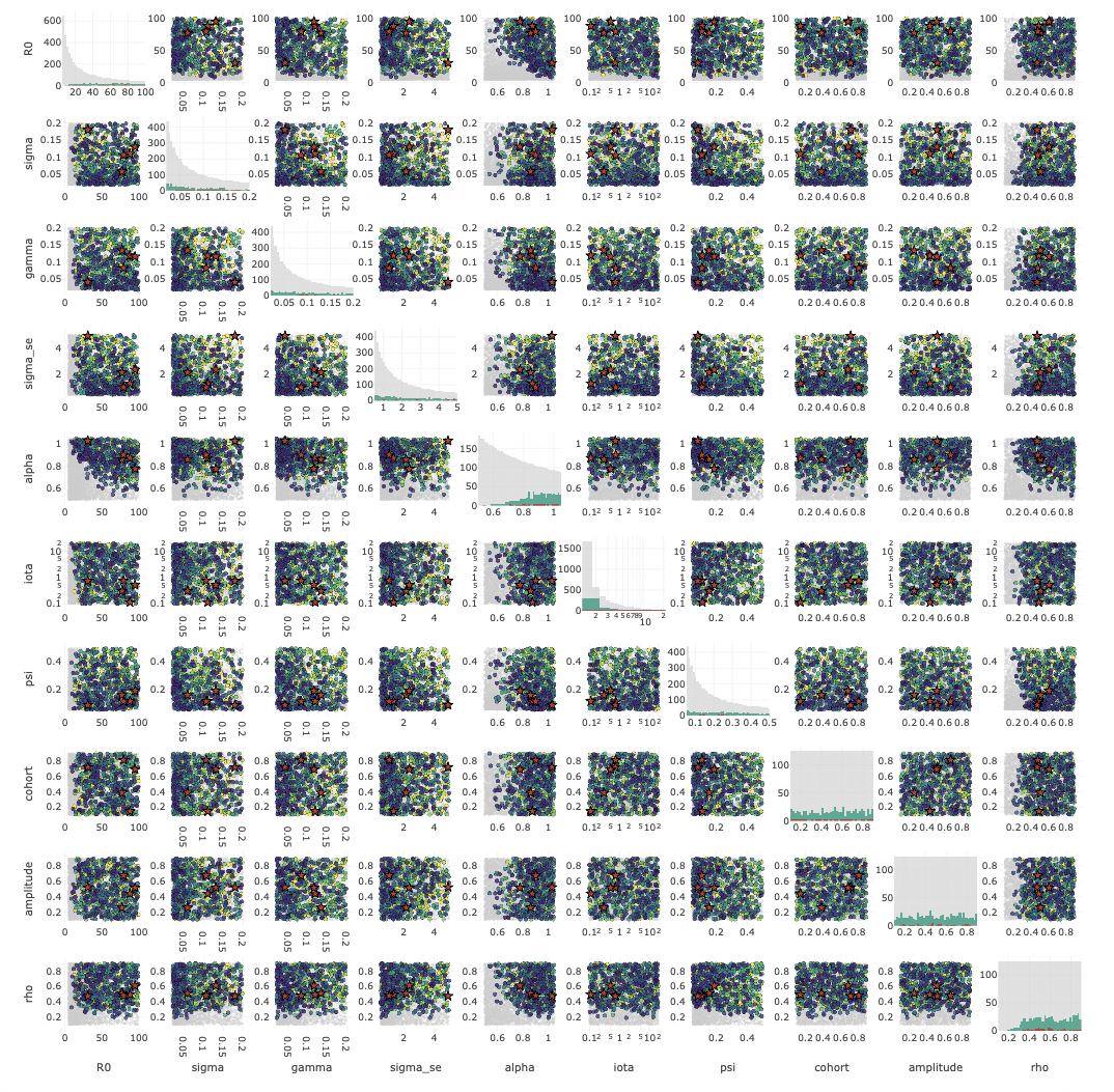
With camdl survey, modelers can see in one figure what would take a day of
mis-spent IF2 runs to discover: which parameters are well-identified, which
trade off in ridges, where the basin actually lives, and whether your bounds
were sensible to begin with. The brightest cluster of points is also a natural
neighborhood to initialize likelihood-based fitting (and camdl makes it easy to
seed its IF2 chains directly from the top-K survey points with init_method = "survey_top_k"). A survey is an exploratory diagnostic, not a fitter; it
doesn’t produce an MLE. But it’s the cheapest hour of compute in the whole
workflow in that it can often prevent hours downstream model fitting
frustrations.
Calibration is a workflow, not a script
Calibrating complicated epi models usually involves hand-assembled script-based pipelines, which can easily grow in both complexity and fragility as multiple models are fit and compared. But with camdl, I wanted to explore ways to build canonical, safer, and more robust calibration pipelines as declarative artifacts:
# fit.toml — the entire calibration pipeline in one file
[model]
camdl = "he2010_london.camdl"

[data.observations]
weekly_cases = "data/cases.tsv"

[holdout]
weekly_cases = "data/cases_holdout.tsv"   # held out, structurally unreachable

[estimate.R0]        bounds = [10, 80]
[estimate.rho]       bounds = [0.3, 0.6]
[estimate.sigma_se]  bounds = [0.05, 0.20]

[stages.scout]
algorithm   = "if2"            # iterated filtering MLE
backend     = "chain_binomial"
chains      = 36
particles   = 2000
iterations  = 200
init_method = "lhs"            # Latin-hypercube starts, scale-aware

[stages.refine]
algorithm   = "pgas"           # Bayesian posterior via PGAS+NUTS
backend     = "chain_binomial"
starts_from = "scout"          # seeds from scout's MLE

[stages.validate]
algorithm = "pfilter"          # held-out predictive log-likelihood
particles = 4000
replicates = 8
The idea of staged fits is that often model-fitting workflows refine
fitting-algorithm knobs as the inference problem goes from broad search to
fit-refinement in a high-likelihood region of parameter space. I wanted a way to
safely integrate this type of workflow into camdl fit run — I emphasize
safely because there’s often an inherent tradeoff between automation and
validation checking.
In order to prevent workflow automation from mindlessly advancing poor fits from one stage to the next, camdl’s staged fits use convergence gates that fail loudly rather than just give faulty results. The scout stage’s gate is two-legged; it must pass both per-parameter chain agreement (Gelman–Rubin-style on IF2’s per-iteration parameter means) and a low decibans spread across chain-level log-likelihoods (indicating all chains ended up in the same high-likelihood basin). Both legs must pass. Early testing (by replicating inference of previously-published results) surfaced that occasionally chains agreed on parameter values yet sat in a basin tens to hundreds of decibans worse than truth — this is the precise failure mode the second leg catches. If either leg of the convergence gates fails, the next “refine” step refuses to start; the user can then fix the underlying issue (widen bounds, more chains, more iterations) rather than the software just advancing results that haven’t converged.
Another fragility surfaced during more early model-fitting testing. I had a
plausible-looking boarding-school SIR
fit
reporting a specific R₀ from a dt=1-day chain-binomial run. At dt=0.1, the same
parameter vector scored 14 nats worse than the dt-converged MLE — the
coarse step had created a phantom basin that the inference loop happily found,
and no in-fit diagnostic at dt=1.0 could catch it (synthetic recovery passes,
because the same dt on both sides cancels the bias). The solution was to
engineer in a Richardson dt-convergence check, which evaluates the converged
log-likelihood over a ladder of halved integrator step sizes (dt, dt/2, dt/4).
The Richardson diagnostic refuses to bless a fit whose likelihood is sensitive
to a finer step size (which it shouldn’t be). This is standard practice in
numerical PDE work but is not, to my knowledge, automated in any epi-fit
pipeline. camdl now runs this check automatically on every fit and emits a
one-line PASS / MARGINAL / FAIL verdict. It complements the L401 lint rather
than duplicating it: L401 catches the fragile AST shape at compile time, while
the Richardson check catches step-size pathology after the fit — which can
arise even from a dt-invariant rate expression.
Returning to the Toyota Production System analogy: jidoka is the idea of stopping the production line the moment an abnormality is detected, so the defect doesn’t reach the next station. Where poka-yoke error-proofs mistakes, jidoka catches them before they propagate; the compiler does the first, the fitting convergence gates do the second. I should again emphasize how important this type of robust engineering is now that coding agents are increasingly writing and fitting more of our modeling code.
Finally, another robustness-engineering feature of camdl is its
content-addressable storage (CAS) system. In command-line scientific work, it’s
somewhat easy for a user to do something like run run-program --x 1 --y 2 --output results/run_x1_y2.tsv, then think “I should try it with y = 3” and run
run-program --x 1 --y 3 --output results/run_x1_y2.tsv. Do you spot the error
here? The underlying issue is that when the modeler is responsible for naming
the output path themselves, they are implicitly responsible for updating the
command call twice; if they forget one, they break the mapping between input
parameters and output results — invalidating everything.
To avoid this class of errors, camdl fit run hashes the full run input —
the canonicalized model IR (stripping whitespace and comments that do not
impact output), parameter values, seed, data files, algorithm config, tool
version — and writes all output to a carefully-designed directory hierarchy
that is keyed on that hash. This also has runtime benefits; if a user re-runs
an expensive fit with an unchanged config, the run input hash would be
identical to a past run and camdl would just say that fit’s already been run.
This prevents the all-too-common issue of a 2-day fit being clobbered by an
accidental re-run or a user forgetting to update the --output path. Instead,
if a user were to change one bit of input, the hash would change too, and a fresh run
starts without touching past results. camdl list enumerates every fit the
project has produced; camdl show <hash> surfaces the exact command and
seed; camdl cat <hash> emits the output. A camdl fit hash is effectively
a citation: paste it into a methods section and any reader with the source
can reproduce the result bit-for-bit. Reproducibility is a property of the
tool, not a discipline left to the user.
The inference stack
I won’t go into much detail on the inference stack here — it deserves its own
series of posts. But the short version is that camdl ships the methods you’d
actually reach for in a serious paper, all driven from the same fit.toml:
- Maximum likelihood via iterated filtering (IF2; Ionides et al., 2015 ), for fast point estimates and likelihood-surface mapping before committing to a full Bayesian run.
- Bayesian posterior sampling via PGAS+NUTS (Lindsten, Jordan & Schön,
2014
; Hoffman & Gelman,
2014
). This allows modelers to
rigorously incorporate expert knowledge through carefully-chosen priors; the
output is posterior samples over parameters and latent states that
automatically propagate uncertainty into decision making. PGAS works well for
long time-series data, which can cause particle degeneration in PMMH. One
fun thing: the gradients NUTS needs fall out as another benefit of camdl’s
compiler architecture: we can use symbolic
differentiation
directly on the expression AST. The OCaml compiler walks each rate expression
and emits the analytical derivative as a source-to-source
rate_gradfield in the IR; the runtime evaluates exact ∇ log ℒ at the cost of one expression-tree walk per step. No autodiff tape, no finite differences, no JAX dependency. The expression language is first-order and pure — the same property that makes the dim-checker tractable also makes symbolic differentiation less than 300 lines of OCaml via its pattern-matching ADT goodness. - Gradient-free fallback via PMMH (Andrieu, Doucet & Holenstein, 2010 ). For shorter time series, problems where symbolic differentiation is blocked, or posterior geometries where NUTS struggles, PMMH is an alternative to PGAS+NUTS.
- Profile likelihoods (Raue et al.,
2009
), both 1D and 2D, are
built-in via the
camdl profilesubcommand. Through a decade of experience fitting fiddly models, I have seen the humble profile likelihood elucidate identifiability problems that would remain hidden behind frustrating, non-converged fits. The value of profiling out a parameter isn’t just about reshaping likelihood geometry to be more optimization/sampler-friendly — in my experience, it’s also an essential part of intuitively understanding one’s model and the data’s informativeness about the model. - Out-of-sample validation via prequential scoring (Dawid, 1984 ; Gneiting & Raftery, 2007 ); built-in held-out predictive performance is the only honest test of fit, and the only honest basis for model comparison.
Here’s a simple example of camdl compare, which allows us to compare the
multiple models that are now cheaper to write and fit with camdl:
$ camdl compare preq_poisson.json preq_negbin.json preq_procnoise.json

Model              T_score     elpd   Δelpd   se(Δ)                evidence   PIT_cov90
─────────────────────────────────────────────────────────────────────────────────────
preq_poisson.json       14   -62.75   -7.44    5.52   -32.3 dB, decisive against    0.71
preq_negbin.json        14   -56.44   -1.12    1.31     -4.9 dB, indeterminate     0.93
preq_procnoise.json     14   -55.32       —       —                          —     0.93

Δelpd is shown relative to the best-supported model (at the bottom); a more-negative Δelpd means worse predictive performance.
Here, the Δelpd column is the expected-log-pointwise-predictive-density gap between an alternative model and the best-supported one (which is in the bottom row; more-negative means worse held-out prediction). The evidence column converts that gap to decibans (10 × log₁₀ of the likelihood ratio, so −10 dB means the data favor the other model by 10:1; see Kass & Raftery 1995 for the conventional “weak / positive / strong / decisive” scale). Finally, the probability-Integral-Transform (PIT) coverage at 90% column shows the fraction of held-out observations whose true value falls inside the model’s 90% predictive interval, which should be near 0.90 for a well-calibrated (in the probabilistic sense) model. In the example above, all three columns are computed from held-out predictive scoring of a simple SEIR fit under two different observation models, and one process noise model. The 0.71 PIT coverage on Poisson flags it as underdispersed; NegBin and the process-noise variant are both well-calibrated at 0.93.
Why a DSL pays off here
Compartmental modeling with camdl is often cheaper than ABMs for many of the
questions epi modelers face. ABMs scale with population × steps × interactions,
and calibration technology is often limited due to the lack of tractable
likelihoods; modelers instead have to resort to ABC, summary-statistic
matching, and repurposing hyperparameter optimizers like Optuna for
calibration. By contrast, camdl scales with parameter count and observation
richness; you get full likelihoods, gradients, posteriors, profile
identifiability checks, and held-out predictive scoring out of the box. For
policy questions where one doesn’t need agent heterogeneity, compartmental
modeling with camdl can mean faster model prototyping — which means that more
model variants can be written and fit in the same wallclock time, and camdl compare allows researchers to choose the best model according to its
performance on held-out data, rather than just assert one is best.
On AI-assisted scientific software
I wrote the camdl alpha release with Claude Code in 974 commits over nine weeks (my first commit was on March 12). I like to do little back-of-the-envelope type calculations to anchor things in relative units that make intuiting these types of numbers easier. So try this exercise, and anchor this pace concretely: the camdl repo is currently ~167,000 lines and ~6.85 MB of source text across OCaml, Rust, Python, Shell, Markdown, and config.
I type about 74 wpm on my laptop keyboard, which is about 22,200 characters per hour. If I personally were to type out the entire repo at my max typing speed, eight hours a day, five days a week, with zero pauses to think, debug, eat, or sleep, it would take ~7.7 work-weeks. The actual elapsed time was ~9 weeks. So even if I had done nothing but transcribe pre-written code at full speed for every working hour of the project, I would have just barely fit it into camdl’s development calendar — with no time left over for higher-level design, debugging, statistical work, or any of the actual engineering. (To be fair, the version of those nine weeks involving no emails, no meetings, and no Teams does have a certain monastic appeal.) At a realistic professional rate for compiler-and-Rust development (somewhere in the 10–50 finished-LoC-per-hour range, since that metric is famously noisy), solo hand-writing this codebase would have taken on the order of 1 to 3 years. When there’s less than twenty years left , we can’t spend 1 to 3 of them just building an easy-to-use, AI-friendly compartmental-modeling DSL — we need to be using it.
So the pace isn’t possible with hand-typing alone, and it raises a question worth answering directly: how do you square AI-assisted development with the engineering rigor, central to camdl’s design, that this post has been arguing for?
Honestly, we don’t yet know. The space of AI-assisted scientific software is too new to have settled norms, and what counts as adequate oversight is now, in many ways, an open empirical question. What I can say is what I tried to do: rapidly de-risk the DSL-with-serious-compiler architecture for stochastic compartmental modeling, and at the same time build a tool that made writing and fitting compartmental models easier (and hopefully fun).
In the last eight months or so I have seen agentic coding tools get incredibly good at writing scientific software, bashing out intricate numerical algorithms carefully and in far less time than I could.3 The bet I made on the engineering side is that lots of planning iteration, using compiled languages with algebraic types (a non-negotiable for me for this type of work), thinking in terms of types (and lots of consolidation refactoring), and 1,204 tests would produce a software product with about the same number of bugs as the average alpha release — and hopefully fewer. The same compiler-checked everything and CI gates that make camdl trustworthy for users are the infrastructure that keeps AI-assisted development in the rigorous mode rather than the vibe-coded one: when the agent gets something wrong, it shows up as a compile error or a failing test, not as a silent bug.
My hope is that this AI-driven workflow I’ve been figuring out was enough to sculpt Claude into something like a second-year grad student that’s really good at coding, overseen in regular meetings by a graduate advisor. I think that’s about where we’re at with the interaction between scientists and AI.
Whether that bet holds up is exactly the kind of thing the field should investigate openly. I actively welcome readers to stress-test this codebase — finding bugs, studying where the agent and I converged on bad design, characterizing what kinds of prompting or test infrastructure would have caught what. The questions about whether AI assistance preserves rigor at this scale matter beyond just camdl, and the work matters to public health.
This generalizes back to the user side, which is where I think it matters most. A scientist using camdl with Anthropic’s Claude Code (the same daily collaborator that made this project possible at this pace) gets the same arrangement I had as the sole developer: the compiler catches what the agent gets wrong, the convergence gates catch what the inference gets wrong, and the modeler is the one whose judgment determines whether the model is the right model for the question.
A specific thanks here to the many, many, Claude Code agents that served me along the way: through these nine weeks Claude has been a daily pair-programmer in OCaml and Rust, a sanity-checker on the statistical derivations, a quick summarizer of methods papers, a partner in debugging the gnarlier corners of the inference stack, and the thing that held a multi-layer codebase in working memory while I focused on any one piece of it. The scientific judgment was mostly mine; the design was something we wove together; the bugs were mostly Claude’s authorship and mine to chase (though I’d have produced a comparable litany on my own — probably more). The engineering tempo this post represents reflects that collaboration.
Try it
This blog post marks camdl’s alpha release — usable for real fits, with a stable enough public surface that we’re documenting it openly, but with breaking changes still expected. If you want to start:
- Read the documentation/vignettes. vsbuffalo.github.io/camdl-docs walks through everything above with executable examples; Getting Started is the entry point.
Send feedback. Source is at github.com/vsbuffalo/camdl . What I most want to hear at this alpha release stage: where the error messages are unhelpful, what camdl language features are missing or feel clunky, where the docs are wrong, what frictions exist during model building and fitting, and which published models you’d want to see reproduced next.
Contribute. camdl is far from feature-complete. Code contributions, model ports, runtime-backend extensions, and stress-testing on real models that surfaces bugs are all welcome. There’s a long backlog of features I’d like camdl to incorporate. Please open an issue or get in touch and I can point you at something that matches your interests.
I’ve had a background interest in compilers and interpreters for a while, since as an undergrad I worked with UC Davis professor and R-core contributor Duncan Temple Lang on RLLVMCompile , an experimental LLVM-based compiler for R. I also caught a brief case of the Lisp bug from Paul Graham’s essays, and wrote a small Lisp interpreter. ↩︎
IDM also has prior art in this genre: CMS , a cool Lisp-like S-expression DSL for compartmental models with several excellent backend solver implementations. I came across it only after starting camdl, so it didn’t shape the design — but it’s the closest in-house precedent and worth knowing about. ↩︎
Though I do miss the sweet, sweet payoff that comes after a week of head-bashing over a numerical underflow, a sign error in the gradient, or a fixed-point iteration that won’t converge — when you finally find the one missing log-sum-exp and the traces snap into agreement with the analytic solution. AI-assisted work does, honestly, trade some of that away. ↩︎